DATABASE MANAGEMENTS PRINCIPLES & APPS

The various types of data models
six types of data models

• 1.ER-Model
• 2.Hierarchical Model
• 3.Network Model
• 4.Inverted Model - ADABAS
• 5.Relational Model
• 6.Object-Oriented Model(s)

1. ER-Model (Entity-Relationship Model)

The Entity - Relationship Model (E-R Model) is a high-level conceptual data model developed by Chen in 1976 to facilitate database design. Conceptual Modeling is an important phase in designing a successful database. A conceptual data model is a set of concepts that describe the structure of a database and associated retrieval and updation transactions on the database. A high level model is chosen so that all the technical aspects are also covered.

The E-R data model grew out of the exercise of using commercially available DBMS's to model the database. The E-R model is the generalization of the earlier available commercial models like the Hierarchical and the Network Model. It also allows the representation of the various constraints as well as their relationships.

So to sum up, the Entity-Relationship (E-R) Model is based on a view of a real world that consists of set of objects called entities and relationships among entity sets which are basically a group of similar objects. The relationships between entity sets is represented by a named E-R relationship and is of 1:1, 1: N or M: N type which tells the mapping from one entity set to another.

The E-R model is shown diagrammatically using Entity-Relationship (E-R) diagrams which represent the elements of the conceptual model that show the meanings and the relationships between those elements independent of any particular DBMS and implementation details.

Features of the E-R Model:

1. The E-R diagram used for representing E-R Model can be easily converted into Relations (tables) in Relational Model.

2. The E-R Model is used for the purpose of good database design by the database developer so to use that data model in various DBMS.

3. It is helpful as a problem decomposition tool as it shows the entities and the relationship between those entities.

4. It is inherently an iterative process. On later modifications, the entities can be inserted into this model.

5. It is very simple and easy to understand by various types of users and designers because specific standards are used for their representation.

ER-Model- Operations

• Several navigational query languages have been proposed
• A closed query language as powerful as relational languages has not been developed
• None of the proposed query languages has been generally accepted

Database Design

Goal of design is to generate a formal specification of the database schema
Methodology:

1. Use E-R model to get a high-level graphical view of essential components of enterprise and how they are related
2. Then convert E-R diagram to SQL DDL, or whatever database model you are using

E-R Model is not SQL based. It's not limited to any particular DBMS. It is a conceptual and semantic model – captures meanings rather than an actual implementation

The E-R Model: The enterprise is viewed as set of

• Entities
• Relationships among entities

Symbols used in E-R Diagram

• Entity – rectangle
• Attribute – oval
• Relationship – diamond
• Link - line

---

Entities and Attributes

Entity: an object that is involved in the enterprise and that be distinguished from other objects. (not shown in the ER diagram--is an instance)

• Can be person, place, event, object, concept in the real world
• Can be physical object or abstraction
• Ex: "John", "CSE305"

Entity Type: set of similar objects or a category of entities; they are well defined

• A rectangle represents an entity set
• Ex: students, courses
• We often just say "entity" and mean "entity type"

Attribute: describes one aspect of an entity type; usually [and best when] single valued and indivisible (atomic)

• Represented by oval on E-R diagram
• Ex: name, maximum enrollment
• May be multi-valued – use double oval on E-R diagram
• May be composite – attribute has further structure; also use oval for composite attribute, with ovals for components connected to it by lines
• May be derived – a virtual attribute, one that is computable from existing data in the database, use dashed oval. This helps reduce redundancy

---

Entity Types

An entity type is named and is described by set of attributes

• Student: Id, Name, Address, Hobbies

Domain: possible values of an attribute.

• Note that the value for an attribute can be a set or list of values, sometimes called "multi-valued" attributes
• This is in contrast to the pure relational model which requires atomic values
• E.g., (111111, John, 123 Main St, (stamps, coins))

Key: subset of attributes that uniquely identifies an entity (candidate key)
Entity Schema: The meta-information of entity type name, attributes (and associated domain), key constraints
Entity Types tend to correspond to nouns; attributes are also nouns albeit descriptions of the parts of entities
May have null values for some entity attribute instances – no mapping to domain for those instances

---

Keys

Superkey: an attribute or set of attributes that uniquely identifies an entity--there can be many of these
Composite key: a key requiring more than one attribute
Candidate key: a superkey such that no proper subset of its attributes is also a superkey (minimal superkey – has no unnecessary attributes)
Primary key: the candidate key chosen to be used for identifying entities and accessing records.  Unless otherwise noted "key" means "primary key"
Alternate key: a candidate key not used for primary key
Secondary key: attribute or set of attributes commonly used for accessing records, but not necessarily unique
Foreign key: term used in relational databases (but not in the E-R model) for an attribute that is the primary key of another table and is used to establish a relationship with that table where it appears as an attribute also.
So a foreign key value occurs in the table and again in the other table. This conflicts with the idea that a value is stored only once; the idea that a fact is stored once is not undermined.

---

Graphical Representation in E-R diagram

Rectangle -- Entity
Ellipses -- Attribute (underlined attributes are [part of] the primary key)
Double ellipses -- multi-valued attribute
Dashed ellipses-- derived attribute, e.g. age is derivable from birthdate and current date.

[Drawing notes: keep all attributes above the entity. Lines have no arrows. Use straight lines only]

---

Relationships

Relationship: connects two or more entities into an association/relationship

• "John" majors in "Computer Science"

Relationship Type: set of similar relationships

• Student (entity type) is related to Department (entity type) by MajorsIn (relationship type).

Relationship Types may also have attributes in the E-R model.  When they are mapped to the relational model, the attributes become part of the relation. Represented by a diamond on E-R diagram.
Relationship types can have descriptive attributes like entity sets
Relationships tend to be verbs or verb phrases; attributes of relationships are again nouns

[Drawing tips: relationship diamonds should connect off the left and right points; Dia can label those points with cardinality; use Manhattan connecting line (horizontal/vertical zigzag)]

---

Attributes and Roles

An attribute of a relationship type describes the relationship

• e.g., "John" majors in "CS" since 2000
• John and CS are related
• 2000 describes the relationship - it's the value of the since attribute of MajorsIn relationship type

The role of a relationship type names one of the related entities
e.g., "John" is value of Student role, "CS" value of Department role of MajorsIn relationship type
(John, CS, 2000) describes a relationship

---

Relationship Type

Relationship types are described by set of roles and [optional] attributes

• e.g., MajorsIn: Student, Department, Since

Think that entities are nouns; relationship types are often verbs

• students and departments are the entities (nouns) and roles in relationship types
• majors is the relationship type (verb)
• i.e., "student" "majors in " "department"

Here we have used as the role name (Student) the name of the entity type (Student) of the participant in the relationship.

---

Degree of relationship

Binary – links two entity sets; set of ordered pairs (most common)
Ternary – links three entity sets; ordered triples (rare)
N-ary – links n entity sets; ordered n-tuples (very rare)
Note: ternary relationships may sometimes be replaced by two binary relationships (see book Figures 3.5 and 3.13). Semantic equivalence between ternary relationships and two binary ones are not necessarily true.

---

Cardinality of Relationships

Number of entity instances to which another entity set can map under the relationship
One-to-one: X-Y is 1:1 when each entity in X is associated with at most one entity in Y, and each entity in Y is associated with at most one entity in X.
One-to-many: X-Y is 1:M when each entity in X can be associated with many entities in Y, but each entity in Y is associated with at most one entity in X.
Many-to-many: X:Y is M:M if each entity in X can be associated with many entities in Y, and each entity in Y is associated with many entities in X ("many" =>one or more and sometimes zero)
 

---

Relationship Participation Constraints

Total participation

• Every member of entity set must participate in the relationship
• Represented by double line from entity rectangle to relationship diamond
• E.g., A Class entity cannot exist unless related to a Faculty member entity

Partial participation

• Not every entity instance must participate
• Represented by single line from entity rectangle to relationship diamond
• E.g., A Textbook entity can exist without being related to a Class or vice versa.

---

Roles

Problem: relationships can relate elements of same entity type
e.g., ReportsTo relationship type relates two elements of Employee entity type:

• Bob reports to Mary since 2000

We do not have distinct names for the roles
It is not clear who reports to whom
Solution: the role name of relationship type need not be same as name of entity type from which participants are drawn

• ReportsTo has roles Subordinate and Supervisor and attribute Since
• Values of Subordinate and Supervisor both drawn from entity type Employee

Optional to name role of each entity, but helpful in cases of

• Recursive relationship – entity set relates to itself
• Multiple relationships between same entity sets

---

Schema of a Relationship Type

Contains the following features:
Role names, R_i, and their corresponding entity sets. Roles must be single valued (the number of roles is called its degree)
Attribute names, A_j, and their corresponding domains. Attributes in the E-R model may be set or multi-valued.
Key: Minimum set of roles and attributes that uniquely identify a relationship
Relationship: 1, …e_n; a₁, …a_k>

• e_i is an entity, a value from R_i’s entity set
• a_j is a set of attribute values with elements from domain of A_j

---

Graphical Representation

Roles are edges labeled with role names (omitted if role name = name of entity set). Most attributes have been omitted.

---

Key Constraint (special case)

If, for a particular participant entity type, each entity participates in at most one relationship, its corresponding role is a foreign key relationship type.

• E.g., Professor role is unique in WorksIn

The representation in an E-R diagram is an arrow.

---

Existence Dependency and Weak Entities

Existence dependency: Entity Y is existence dependent on entity X is each instance of Y must have a corresponding instance of X
In that case, Y must have total participation in its relationship with X
If Y does not have its own candidate key, Y is called a weak entity, and X is strong entity
Weak entity may have a partial key, called a discriminator, that distinguishes instances of the weak entity that are related to the same strong entity
Use double rectangle for weak entity, with double diamond for relationship connecting it to its associated strong entity
Note: not all existence dependent entities are weak – the lack of a key is essential to definition

ER Diagram Example

2.Hierarchical Model

   

What is DBMS Hierarchical Model?

    Hierarchical data base Model is used to represent the data in a tree like structure.

Hierarchical data base is organized in to a tree like structure implying a single upward link in each record to describe the nesting and a sort field to keep the records in a particular order in each same level list.

• The hierarchical data model organizes data in a tree structure.
• There is a hierarchy of parent and child data segments.
• This structure implies that a record can have repeating information, generally in the child data segments.
• Data in a series of records, which have a set of field values attached to it.
• It collects all the instances of a specific record together as a record type.

Types of DBMS languages

Data Definition Language-DDL

Data Definition Language (DDL) statements are used to define the database structure or schema. 

Some examples: 

CREATE - to create objects in the database

ALTER - alters the structure of the database

DROP - delete objects from the database

TRUNCATE - remove all records from a table, including all spaces allocated for the records are removed

COMMENT - add comments to the data dictionary

RENAME - rename an object

---

Data Manipulation Language (DML)

Data Manipulation Language (DML) statements are used for managing data within schema objects. 

Some examples: 

SELECT - Retrieve data from the a database

INSERT - Insert data into a table

UPDATE - Updates existing data within a table

DELETE - deletes all records from a table, the space for the records remain

MERGE - UPSERT operation (insert or update)

CALL - Call a PL/SQL or Java subprogram

EXPLAIN PLAN - explain access path to data

LOCK TABLE - control concurrency

---

Data Control Language (DCL)

Data Control Language (DCL) statements. 

Some examples: 

GRANT - gives user's access privileges to database

REVOKE - withdraw access privileges given with the GRANT command

---

Transaction Control (TCL)

Transaction Control (TCL) statements are used to manage the changes made by DML statements. It allows statements to be grouped together into logical transactions. 

Some examples: 

COMMIT - save work done

SAVEPOINT - identify a point in a transaction to which you can later roll back

ROLLBACK - restore database to original since the last COMMIT

SET TRANSACTION - Change transaction options like isolation level and what rollback segment to use

Codd's 12 Rules for RDBMS

• The Information rule
• The Guaranteed Access rule
• The Systematic Treatment of Null Values rule
• The Dynamic Online Catalog Based on the Relational Model rule
• The Comprehensive Data Sublanguage rule
• The View Updating rule
• The High-level Insert, Update, and Delete rule
• The Physical Data Independence rule
• The Logical Data Independence rule
• The Integrity Independence rule
• The Distribution Independence rule
• The No subversion rule
• GO TO DIRECT LINK....of DBMS

Record

A collection of field or data items values that provide information on an entity. Each field has a certain data type such as integer, real or string. Record of the same type are group into record type.

Parent Child Relationship Type

It is 1:N relation between two record type. The record type 1 side is parent record type and one on the N side is called child record type of the PCR type.

Advantages

1.Simplicity

Data naturally have hierarchical relationship in most of the practical situations. Therefore, it is easier to view data arranged in manner. This make this type of database more suitable for the purpose.

2.Security

These database system can enforce varying degree of security feature unlike flat-file system.

3.Database Integrity

Because of its inherent parent-child structure, database integrity is highly promoted in these system.

Disadvantages

1.Complexity of Implementation

The actual implementation of a hierarchical database depends on the physical storage of data. This makes the implementation complicated.

2.Difficulty in Management

The movement of a data segment from one location to another causes all the accessing programs to be modified making database management a complex affair.

3.Complexity of Programming

Programming a hierarchical database is relatively complex because the programmers must know the physical path of the data items.

4.Poor Portability

The database are not easily portable mainly because there is little or no standard existing for these types of database. 

3.Network Model
   
  Network model is a collection data in which records are physically linked through linked lists .
A DBMS is said to be a Network DBMS if the relationships among data in the database are of type many-to-many. The relationships among many-to-many appears in the form of a network. Thus the structure of a network database is extremely complicated because of these many-to-many relationships in which one record can be used as a key of the entire database. A network database is structured in the form of a graph that is also a data structure .



                                  Figure above is an Example of Network Model.
The network model is a database model conceived as a flexible way of representing objects and their relationships. Its distinguishing feature is that the schema, viewed as a graph in which object types are nodes and relationship types are arcs, is not restricted to being a hierarchy or lattic.

Database systems

Some well-known database systems that use the network model include:

• Digital Equipment corporation DBMS-10
• Digital Equipment Corporation DBMS-20
• Digital Equipment Corporation VAX DBMS
• Honeywell IDS (Integrated Data Store)
• IDMS (Integrated Database Management System)
• RDM Embedded
• RDM Server
• TurboIMAGE
• Univac DMS-1100

4. INVERTED MODELS

     
       In computer science, an inverted index (also referred to as postings file or inverted file) is an index data structure storing a mapping from content, such as words or numbers, to its locations in a database file, or in a document or a set of documents. The purpose of an inverted index is to allow fast full text searches, at a cost of increased processing when a document is added to the database. The inverted file may be the database file itself, rather than its index. It is the most popular data structure used in document retrieval systems, used on a large scale for example in search engines. Several significant general-purpose mainframe-based database management systems have used inverted list architectures, including ADABAS, DATACOM/DB, and Model 204.
There are two main variants of inverted indexes: A record level inverted index (or inverted file index or just inverted file) contains a list of references to documents for each word. A word level inverted index (or full inverted index or inverted list) additionally contains the positions of each word within a document. The latter form offers more functionality (like phrase searches), but needs more time and space to be created.

Example

Given the texts "it is what it is", "what is it" and "it is a banana", we have the following inverted file index (where the integers in the set notation brackets refer to the subscripts of the text symbols, ,  etc.):

"a":      {2}
"banana": {2}
"is":     {0, 1, 2}
"it":     {0, 1, 2}
"what":   {0, 1}

A term search for the terms "what", "is" and "it" would give the set .

With the same texts, we get the following full inverted index, where the pairs are document numbers and local word numbers. Like the document numbers, local word numbers also begin with zero. So, "banana": {(2, 3)} means the word "banana" is in the third document (), and it is the fourth word in that document (position 3).

"a":      {(2, 2)}
"banana": {(2, 3)}
"is":     {(0, 1), (0, 4), (1, 1), (2, 1)}
"it":     {(0, 0), (0, 3), (1, 2), (2, 0)} 
"what":   {(0, 2), (1, 0)}

If we run a phrase search for "what is it" we get hits for all the words in both document 0 and 1. But the terms occur consecutively only in document 1.

[edit]Applications

The inverted index data structure is a central component of a typical search engine indexing algorithm. A goal of a search engine implementation is to optimize the speed of the query: find the documents where word X occurs. Once a forward index is developed, which stores lists of words per document, it is next inverted to develop an inverted index. Querying the forward index would require sequential iteration through each document and to each word to verify a matching document. The time, memory, and processing resources to perform such a query are not always technically realistic. Instead of listing the words per document in the forward index, the inverted index data structure is developed which lists the documents per word.

With the inverted index created, the query can now be resolved by jumping to the word id (via random access) in the inverted index.

In pre-computer times, concordances to important books were manually assembled. These were effectively inverted indexes with a small amount of accompanying commentary that required a tremendous amount of effort to produce.

In bioinformatics, inverted indexes are very important in the sequence assembly of short fragments of sequenced DNA. One way to find the source of a fragment is to search for it against a reference DNA sequence. A small number of mismatches (due to differences between the sequenced DNA and reference DNA, or errors) can be accounted for by dividing the fragment into smaller fragments—at least one subfragment is likely to match the reference DNA sequence. The matching requires constructing an inverted index of all substrings of a certain length from the reference DNA sequence. Since the human DNA contains more than 3 billion base pairs, and we need to store a DNA substring for every index, and a 32-bit integer for index itself, the storage requirement for such an inverted index would probably be in the tens of gigabytes, just beyond the available RAM capacity of most personal computers today.

6.Object-Oriented Model

Data Modeling PPT...Click to directly Link

SUMMARY OF DBMS MODELS

The various database models

Databases appeared in the late 1960s, at a time when the need for a flexible information management system had arisen. There are five models of DBMS, which are distinguished based on how they represent the data contained:

• The hierarchical model: The data is sorted hierarchically, using a downward tree. This model uses pointers to navigate between stored data. It was the first DBMS model.
  
• The network model: like the hierarchical model, this model uses pointers toward stored data. However, it does not necessarily use a downward tree structure. 
  
• The relational model (RDBMS, Relational database management system): The data is stored in two-dimensional tables (rows and columns). The data is manipulated based on the relational theory of mathematics. 
  
• The deductive model: Data is represented as a table, but is manipulated using predicate calculus.
• The object model (ODBMS, object-oriented database management system): the data is stored in the form of objects, which are structures called classes that display the data within. The fields are instances of these classes 
  

By the late 1990s, relational databases were the most commonly used (comprising about three-quarters of all databases).

DATA MODELING OVERVIEWS
Introduction
To begin our discussion of data models we should first begin with a common understanding of what exactly we mean when we use the term. A data model is a picture or description which depicts how data is to be arranged to serve a specific purpose. The data model depicts what that data items are required, and how that data must look. However it would be misleading to discuss data models as if there were only one kind of data model, and equally misleading to discuss them as if they were used for only one purpose. It would also be misleading to assume that data models were only used in the construction of data files.
Some data models are schematics which depict the manner in which data records are connected or related within a file structure. These are called record or structural data models. Some data models are used to identify the subjects of corporate data processing - these are called entity-relationship data models. Still another type of data model is used for analytic purposes to help the analyst to solidify the semantics associated with critical corporate or business concepts.
The record data modelThe record version of the data model is used to assist the implementation team by providing a series of schematics of the file that will contain the data that must be built to support the business processing procedures. When the design team has chosen a file management system, or when corporate policy dictates that a specific data management system, these models may be the only models produced within the context of a design project. If no such choice has been made, they may be produced after first developing a more general, non-DBMS specific entity relationship data model.
These record data model schematics may be extended to include the physical parameters of file implementation, although this is not a prerequisite activity. These data models have much the same relationship to the building of the physical files and program specifications have to the program code produced by the programmers. In these cases, the data analysis activities are all focused on developing the requirements for and specifications of those files.
These models are developed for the express purpose of describing the "structure of data".
This use of the term presupposes that data has a structure. If we assume for the moment that data has a structure, or that data can be structured, what would it look like. For that matter what does data look like? The statement also presupposes that there is one way, or at least a referred way to model data.
Practically speaking however these models depict the "structure" or logical schematic of the data records as the programmer must think of them, when designing the record access sequences or navigational paths through the files managed by the data management systems.
With the above as an introduction, we can begin a discussion of data and data models. We will use the above as a common starting point, and a common perspective.
Early data modelsAlthough the term data modeling has become popular only in recent years, in fact modeling of data has been going on for quite a long time. It is difficult for any of us to pinpoint exactly when the first data model was constructed because each of us has a different idea of what a data model is. If we go back to the definition we set forth earlier, then we can say that perhaps the earliest form of data modeling was practiced by the first persons who created paper forms for collecting large amounts of similar data. We can see current versions of these forms everywhere we look. Every time we fill out an application, buy something, make a request on using anything other than a blank piece of paper or stationary, we are using a form of data model.
These forms were designed to collect specific kinds of information, in specific format. The very definition of the word form confirms this.
A definition

A form is the shape and structure of something as distinguished from its substance. A form is a document with blanks for the insertion of details or information.

Almost all businesses and in fact almost all organization use forms of every sort to gather and store information.
Why are forms used? A form is used to ensure that the data gathered by the firm is uniform (always the same, consistent, without variation) and can thus be organized and used for a variety of different purposes. The form can be viewed as a schematic which tells the person who is to fill it out what data is needed and where that data is to be entered. Imagine if you will what would happen if the firm's customer orders arrived in a haphazard manner, that is, in any way the customer thought to ask. Most of the orders would take a long time to interpret and analyze, much of the information that the firm needed to process the order would probably be missing, or at best be marginally usable by the firm.
In many firms, especially those who receive a large number of unsolicited orders, a large amount of time is spent in trying to figure out what the customer wanted, and whether in fact the customer was ordering one of the firm's products at all.
This is in contrast to those firms where orders come in on preprinted order forms of the company's design. While this doesn't ensure that the customer will fill out the form correctly at least there is the hope that the firm has communicated what it wants and needs.
Forms and automationAs firms began to use automation to process their data, it became more and more important to gather standardized data. Early computing machinery had little if any ability to handle data that was not uniform. Data was taken from the paper record forms and punched into card records which were then fed into machines. Machines that had minimal (by today's standards) logic capability. These machines performed the mechanical functions of totaling, sorting, collating and printing data but had little ability to edit that data. In fact these machines were highly sensitive to data which was not exactly in the expected form.
The card records to which the data was transferred for machine processing were initially designed to follow the sequence of data as it appeared on the form. New forms were designed on which the analyst could layout or structure the data fields (the components of the automated records) on the cards. Additional forms were designed to assist the analyst in designing the reports to be produced from that data. This process of designing card record and report layouts was probably the earliest examples of data modeling.
Although the media dictated the length constraints of the data entry and storage records (mainly 80 column cards), the analysts had some latitude within those constraints. The amount of data to be entered from a given form dictated the number of card records needed. The number of cards and the complexity of the data placed further constraints on the card layouts, the number of columns available, and the positioning of the fields on each card. Further constraints were imposed by the mechanical processing that had to be performed (sorting, merging, collating of cards) requiring control fields, sequence fields, and fields for identifying specific card formats. Multiple card formats were used to accommodate different kinds of data cards - name and address cards, account balance cards, order item cards, etc.
The influence of magnetic tape mediaThe introduction of magnetic tape media removed many of the constraints of size from data record layouts, but left many of the field sequence and record identification requirements. Although new record layout techniques were being developed, many of the early magnetic record layouts looked remarkably similar to their predecessor cards. Magnetic tape media also reduced the number of record format indicators needed to identify the various types and layouts of records. As experience with magnetic tape media increased many analysts experimented with larger and larger records, and introduced more descriptive data to accompany the process support data in the original files. This descriptive data allowed systems designers to provide more meaningful data to the business users.
Tape also allowed data to be more easily sorted, and data from multiple files to be merged and collated. Because of its ease of use and high capacity, many critical processing systems were, and still are based on tape based files.
Tape however still retained several limitations:

1. Tape could not be modified in place. Maintenance of data stored on tape required the old data to be read in, modified in machine memory and new records written out on a new tape. This type of "old master - new master" processing is still in use today.
2. Tape records could not be retrieved randomly or selectively. The sequential storage of records on tape required that the tape be read from beginning to end every time data was needed, even when the data needed constituted only a small part of the file.
3. Modification of tape based data records was achieved by adding fields on to the end of the record layout.
4. Although tape storage introduced the concept of variable length records, and in some cases variable length data fields, processing of those files was cumbersome, and resource intensive, and placed additional restrictions on the mechanical aspects of processing such as sorting, etc. Because of this most tape processing was restricted to fixed length, fixed field record layouts. This restricted the manner in which repetitive, but variable occurrence data could be handled.For instance, retention of monthly data required either one tape per month to be generated, thus requiring multiple tapes to be read to accumulate multi-month reports or month to month comparisons, or provisions had to be made within the tape record for monthly fields (commonly called "buckets") in which case depending upon the month one or more "buckets" would be empty or filled. The designer however had to make these layout choices during the design phase and then develop the processing procedures to accommodate that design choice.

Direct Access file storageAlmost concurrently with the introduction of tape record storage, the vendors introduced another magnetic storage media - commonly called disk or Direct Access Storage Devices (DASD). This form of media used rotating or spinning drums (a form that never really became popular because of its limited capacity and large size) or platters coated with magnetic material to store data, and used moveable arms equipped with heads for reading and writing data to the media.
The early versions of these devices were faster than tape, and allowed for direct access to data (facilitated by the moveable arms) but had fixed capacity which was much smaller than that of the tape units of the same period.
Although these devices allowed for greater processing flexibility early record design techniques for them was almost identical those used for tape records.
These devices however allowed vendors to develop and introduce additional methods of storing and accessing data based on the direct and random processing capabilities. These devices allowed data to be located based on physical media address and thus indices could be constructed which allowed for both sequential and random processing. These addresses also permitted various records to be tied together using the physical address as "pointers" from record to record. The standard vendor-supplied file access mechanisms however still required that all records in a given file have the same layout. Because the record access was relatively fixed, and because the record layouts were also relatively fixed there was no real need for a data model as such since all that was really necessary was to know what fields were contained in each record and to understand what order the fields appeared.
Data Management SystemsUntil the introduction of data management systems (and data base management systems) data modeling and data layout were synonymous. With one notable exception data files were collections of identically formatted records. That exception was a concept introduced in card records - the multi-format-card set, or master detail set. This form of card record layout within a file allowed for repeating sets of data within specific a larger record concept - the so-called logical record (to distinguish it from the physical record). This form was used most frequently when designing files to contain records of orders, where each order could have certain data which was common to the whole order (the master) and individual, repetitive records for each order line item (the details). This method of file design employed record fragmentation rather than record consolidation.
To facilitate processing of these multi-format record files, designers used record codes to identify records with different layouts and redundant data to permit these records to be collected (or tied) together in sequence for processing. Because these files were difficult to process, the layout of these records, and the identification and placement of the control and redundant identifier data fields had to be carefully planned. The planning and coordination associated with these kinds of files constituted the first instances of data modeling.
The concepts associated with these kinds of files were transferred to magnetic media and expanded by vendors who experimented with the substitution of physical record addresses for the redundant data. This use of physical record addresses coupled with various techniques for combining records of varying lengths and formats gave rise to products which allowed for the construction of complex files containing multiple format records tied together in complex patterns to support business processing requirements.
These patterns were relatively difficult to visualize and schematics were devised to portray them. These schematics were also called data models because they modeled how the data was to be viewed. Because the schematics were based on the manner in which the records were physically tied together, and thus logically accessed, rather than how they were physically arranged on the direct access device, they were in reality data file structure models, or data record structure models. Over time the qualifications to these names became lost and they became simply known as data models.
Whereas previously data was collected into large somewhat haphazardly constructed records for processing, these new data management systems allowed data to be separated into smaller, more focused records which could be tied together to form a larger record by the data management system. The this capability forced designers to look at data in different ways.
Data management modelsThe data management systems (also called data base management systems) introduced several new ways of organizing data. That is they introduced several new ways of linking record fragments (or segments) together to form larger records for processing. Although many different methods were tried, only three major methods became popular: the hierarchic method, the network method, and the newest, the relational method.
Each of these methods reflected the manner in which the vendor constructed and physically managed data within the file. The systems designer and the programmer had to understand these methods so that they could retrieve and process the data in the files. These models depicted the way the record fragments were tied to each other and thus the manner in which the chain of pointers had to be followed to retrieved the fragments in the correct order.
Each vendor introduced a structural model to depict how the data was organized and tied together. These models also depicted what options were chosen to be implemented by the development team, data record dependencies, data record occurrence frequencies, and the sequence in which data records had to be accessed - also called the navigation sequence.
The hierarchic modelThe hierarchic model (figure 7-1) is used to describe those record structures in which the various physical records which make up the logical record are tied together in a sequence which looks like an inverted tree. At the top of the structure is a single record. Beneath that are one or more records each of which can occur one or more times. Each of these can in turn have multiple records beneath them. In diagrammatic form the top to bottom set of records looks like a inverted tree or a pyramid of records. To access the set of records associated with the identifier one started at the top record and followed the pointers from record to record.

The various records in the lower part of the structure are accessed by first accessing the records above them and then following the chain of pointers to the records at the next lower level. The records at any given level are referred to as the parent records and the records at the next lower level that are connected to it, or dependent on it are referred to as its children or the child records. There can be any number of records at any level, and each record can have any number of children. Each occurrence of the structure normally represent the collection of data about a single subject. This parent-child repetition can be repeated through several levels.
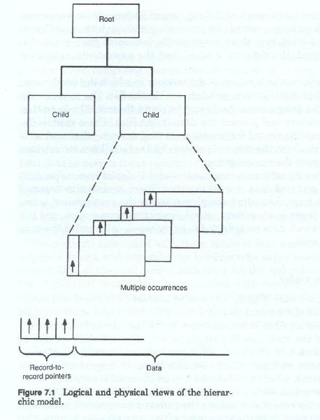
The data model for this type of structural representation usually depicts each segment or record fragment only once and uses lines to show the connection between a parent record and its children. This depiction of record types and lines connecting them looks like an inverted tree or an organizational hierarchy chart.
Each file is said to consist of a number of repetitions of this tree structure. Although the data model depicts all possible records types within a structure, in any given occurrence, record types may or may not be present. Each occurrence of the structure represents a specific subject occurrence an is identified by a unique identifier in the single, topmost record type (the root record).
Designers employing this type of data management system would have to develop a unique record hierarchy for each data storage subject. A given application may have several different hierarchies, each representing data about a different subject, associated with it and a company may have several dozen different hierarchies of record types as components of its data model. A characteristic of this type of model is that each hierarchy is normally treated as separate and distinct from the other hierarchies, and various hierarchies can be mixed and matched to suit the data needs of the particular application.
The network modelThe network data model (figure 7-2) has no implicit hierarchic relationship between the various records, and in many cases no implicit structure at all, with the records seemingly placed at random. The network model does not make a clear distinction between subjects mingling all record types in an overall schematic. The network model may have many different records containing unique identifiers, each of which acts as an entry point into the record structure. Record types are grouped into sets of two, one or both of which can in turn be part of another set of two record types. Within a given set, one record type is said to be the owner record and one is said to be the member record. Access to a set is always accomplished by first locating the specific owner record and then following the chain of pointers to the member records of the set. The network can be traversed or navigated by moving from set to set. Various different data structures can be constructed by selecting sets of records and excluding others.
Each record type is depicted only once in this type of data model and the relationship between record types is indicated by a line between them. The line joining the two records contains the name of the set. Within a set a record can have only one owner, but multiple owner member sets can be constructed using the same two record types
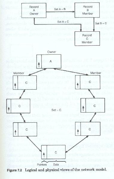
The network model has no explicit hierarchy and no explicit entry point. Whereas the hierarchic model has several different hierarchies structures, the network model employs a single master network or model, which when completed looks like a web of records. As new data is required, records are added to the network and joined to existing sets.
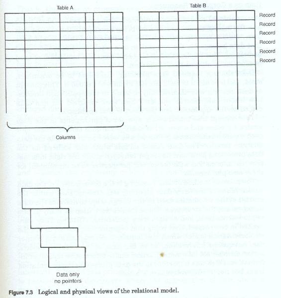
The relational modelThe relational model (figure 7-3), unlike the network or the hierarchic models did not rely on pointers to connect and chose to view individual records in sets regardless of the subject occurrence they were associated with. This is in contrast to the other models which sought to depict the relationships between record types. In the network model records are portrayed as residing in tables with no physical pointer between these tables. Each table is thus portrayed independently from each other table. This made the data model itself a model of simplicity, but it in turn made the visualization of all the records associated with a particular subject somewhat difficult.
Data records were connected using logic and by using that data that was redundantly stored in each table. Records on a given subject occurrence could be selected from multiple tables by matching the contents of these redundantly stored data fields.
The impact of data management systemsThe use of these products to manage data introduced a new set of tasks for the data analysis personnel. In addition to developing record layouts, they also had the new task of determining how these records should be structured, or arranged and joined by pointer structures.
Once those decisions were made they had to be conveyed to the members of the implementation team. The hierarchic and network models were necessary because without them the occurrence sequences and the record to record relationships designed into the files could not be adequately portrayed. Although the relational "model" design choices also needed to be conveyed to the implementation team, the relational model was always depicted in much the same format as standard record layouts, and any other access or navigation related information could be conveyed in narrative form.
Data as a corporate Resource
One additional concept was introduced during the period when these new file management systems were being developed - the concept that data was a corporate resource. The implications of concept were that data belonged to the corporation as a whole, and not to individual user areas. This implied that data should somehow be shared, or used in common by all members of the firm.
Data sharing required data planning. Data had to be organized, sized and formatted to facilitate use by all who needed it. This concept of data sharing was diametrically opposed to the application orientation where data records and data files were designed for, and data owned by the application and the users of that application.
This concept also introduced a new set of participants in the data analysis process and a new set of users of the data models. These new people were business area personnel who were now drawn into the data analysis process. The data record models which had sufficed for the data processing personnel no longer conveyed either the right information nor information with the correct perspective to be meaningful for these new participants.
The primary method of data planning is the development of the data model. Many of the early data planning was accomplished within the context of the schematics used by the design team to describe the data management file structures.
These models were used as analysis and requirements tools, and as such were moderately effective. They were limited in one respect, that being that organizations tended to use the implementation model, which also contained information about pointer use, navigation information, or in the case of the network models, owner-member set information, access choice information and other information which was important to the data processing implementation team, but not terribly relevant to the user.
NormalizationConcurrent with the introduction of the relational data model another concept was introduced - that of normalization. Although it was introduced in the early nineteen-seventies its full impact did not begin to be felt until almost a decade later, and even today its concepts are not well understood. The various record models gave the designer a way of presenting to the user not only the record layout but also also the connections between the data records. In a sense allowing the designer to show the user what data could be accessed with what other data. Determination of record content however was not addressed in any methodical manner. Data elements were collect into records in a somewhat haphazard manner. That is there was no rationale or predetermined reason why one data element was placed in the same record as another. Nor was there any need to do so since the physical pointers between records prevented data on one subject from being confused with data about another, even at the occurrence level.
The relational model however lacked these pointers and relied on logic to assemble a complete set of data from its tables. Because it was logic driven (based upon mathematics) the notion was proposed that placement of data elements in records could also be guided by a set of rules. If followed, these rules would eliminate many of the design mistakes which arose from the meaning of data being inadvertently changed due to totally unrelated changes. It also set forth rules which if followed would arrange the data within the records and within the files more logically and more consistently.
Previously data analysis, file and record designers, relied on intuition and experience to construct record layouts. As the design progressed, data was moved from record to record, records were split and others combined until the final model was pleasing, relatively efficient and satisfied the processing needs of the application that needed the data that these models represented. Normalization offered the hope that the process of record layout, and thus model development could be more procedurally driven, more rule driven such that relatively inexperienced users could also participate in the process. It was also hoped that these rules would also assist the experienced designer and eliminate some of the iterations, and thus make the process more efficient.
The first rule of normalization was that data should depend (or be collected) by key. That is, data should be organized by subject, as opposed to previous methods which collected data by application or system. This notion was obvious to hierarchic model users, whose models inherently followed this principle, but was somewhat foreign and novel to network model developers where the aggregation of data about a data subject was not as commonplace.
This notion of subject organized data led to the development of non-DBMS oriented data models.
The Entity-Relationship modelWhile the record data models served many purposes for the system designers, these models had little meaning or relevance to the users community. Moreover, much of the information the users needed to evaluate the effectiveness of the design was missing. Several alternative data model formats were introduced to fill this void. These models attempted to model data in a different manner. Rather than look at data from a record perspective, they began to look at the entities or subjects about which data was being collected and maintained. They also realized that the the relationship between these data subjects was also an area that needed to be modeled and subjected to user scrutiny. These relationships were important because in may respects they reflected the business rules under which the firm operated. This modeling of relationships was particularly important when relational data management systems were being used because the relationship between the data tables was not explicitly stated, and the design team required some method for describing those relationships to the user.
As we shall see later on, the Entity-Relatinship model has one other important advantage. In as much as it is non-DBMS specific, and is in fact not a DBMS model at all, data models can be developed by the design team without first having to make a choice as to which DBMS to use. In those firms where multiple data management systems are both in use and available, this is a critical advantage in the design process.